The curse of dimensionality comes into play when we deal with a lot of data having many dimensions or features. The dimension of the data is the number of characteristics or columns in a dataset.
High-dimensional data has several challenges, the most notable of which is that it becomes extremely difficult to find meaningful correlations while processing and visualizing it. In addition, as the number of dimensions increases, training the model becomes much slower. More dimensions invite more chances for multicollinearity as well. Multicollinearity is a condition in which two or more variables are found to be highly correlated with one another.
What is the curse of dimensionality?
The curse of dimensionality is a term used to describe the issues when classifying, organizing, and analyzing high-dimensional data, particularly data sparsity and “closeness” of data.
Why is it a curse?
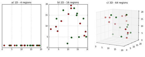
Data sparsity is an issue that arises when you go to higher dimensions. Because the amount of space represented grows so quickly that data can’t keep up, it becomes sparse, as seen below. The sparsity problem is a big issue for statistical significance. As the data space approaches two dimensions and then three dimensions, the amount of data filling it decreases. As a consequence of this, the data for analysis grows dramatically.

Consider a data set with four points in one dimension (only one feature in the data set). It may be simply represented using a line, and the dimension space is equal to 4 since there are only four data points. Suppose we include another feature, which results in a 4-dimensional increase in space. If we add one more component to it, the space will expand to 16 dimensions. Dimensions space grows exponentially as the number of dimensions rises.

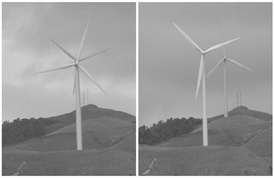
The second issue is how to sort or classify the data. Data may appear similar in low-dimensional spaces, but as the dimension increases, these data points may seem more distant. In the image above, two dimensions appear close together but look distant when viewed in three dimensions. The curse of dimensionality has the same effect on data.
With the increase in the dimensions, the calculating distance between observations becomes increasingly difficult, and all algorithms that rely on correlation calculate it to be an uphill struggle.
More dimensions require more training
Neural networks are instantiated with a certain number of features (dimensions). Each data has its own set of characteristics, each one falling somewhere along a dimension. We may want one feature to handle color, for example, while another handles weight. Each feature adds information, and if we could comprehend every feature conceivable, we would be able to accurately convey which fruit we are thinking about. However, an infinite number of features necessitates infinite training instances, thereby rendering our network’s real-world usefulness doubtful.
The amount of training data required grows drastically with each new feature. Even if we only had 15 features, each being a ‘yes’ or ‘no’ question, the number of training samples needed would be 21532,000.

When does the curse of dimensionality take effect?
The following are just a few examples of domains where the direct consequence of the curse of dimensionality may be observed: Machine learning takes the worst hit from the curse.
Machine Learning
In Machine Learning, a marginal increase in dimensionality necessitates a substantial expansion in the amount of data to maintain comparable results. The by-product of a phenomenon that occurs with high-dimensional data is the curse of dimensionality.
Anomaly Detection
Anomaly detection is finding unusual items or events in the data. In high-dimensional data, anomalies frequently have many irrelevant attributes; various things appear more often in neighbor lists than others.
Combinatorics
When there are more possibilities for input combinations, the complexity grows quickly, and the curse of dimensionality strikes.
Mitigating the curse of dimensionality
To deal with the curse of dimensionality caused by high-dimensional data, a collection of methods known as “Dimensionality Reduction Techniques” is employed. Dimensionality reduction procedures are divided into “Feature selection” and “Feature extraction.”
Feature selection Techniques
The features are evaluated for usefulness and then chosen or eliminated in feature selection methods. The following are some of the most popular Feature selection procedures.
- Low Variance filter: The variance in the distribution of all variables in a dataset is compared, and those with very low variation are removed in this method. Attributes with a little variance will be nearly constant; thus, they won’t help the model’s predictability.
- High Correlation filter: The correlation between attributes is evaluated in this method. The most correlated pair of features are deleted, and the other is kept. The retained one records the degree of difference in the eliminated feature.
- Multicollinearity: When attributes are highly correlated, a high degree of precision may not be obtained for pairs of characteristics, but if each attribute is regressed as a function of the others, we may observe that some of the attributes’ variances are completely covered by the others. The multicollinearity problem is corrected by removing attributes with high VIF values generally greater than 10. High VIF values indicate that there may be a lot of redundancy between related variables and can cause instability in a regression model.
- Feature Ranking: Decision trees and similar models, such as CART, can rank attributes based on their importance or contribution to the model’s predictability. In high-dimensional data, certain of the lower-ranking variables may be removed to reduce the number of dimensions.
- Forward selection: When using high-dimensional data in constructing multi-linear regression models, a method may be used where only one attribute is chosen to start. The final characteristics are added individually, and their value is verified with “Adjusted-R2” values. If the Adjusted-R2 value increases significantly, the variable is kept; otherwise, it is eliminated.
Feature Extraction Techniques
The high-dimensional features are combined into low-dimensional components (PCA or ICA) or factored into low-dimensional components (FA).
- Principal Component Analysis (PCA): The Principal Component Analysis (PCA) is a dimensionality reduction technique in which high-dimensional correlated data is converted to a lower-dimensional set of uncorrelated components known as principal components. The reduced-dimension principal components account for most of the information in the original high-dimensional dataset. A ‘n’-dimensional data set is transformed into ‘n’ fundamental components, with a subset of the ‘n’ principle components being chosen based on the percentage of variance in the data that is to be captured through the principles.
- Factor Analysis (FA): Factor analysis assumes that all of the observed characteristics in a dataset can be represented as a weighted linear combination of latent factors. The thinking behind this approach is that an ‘n-dimensional data might be modeled with ‘m’ components (m<n). The primary distinction between PCA and FA is that While PCA combines the base attributes,
- Independent Component Analysis (ICA): The foundation of the ICA assumption is that all attributes are made up of independent components and that these variables are broken down into a mix of these components.PCA is more resilient than CCA and is most often utilized when PCA and FA fail.


