Dimensionality reduction as means of feature extraction
Feature extraction is a very broad and essential area of data science. It’s goal is to take out salient and informative features from input data, so that they can be used further in predictive algorithms. Modern data scientists observe large amounts of data, which is hard to process at once: data can be raw, unstructured, high dimensional, or noisy. Thus, extracting salient features is vital for successful applications of machine learning algorithms. Feature extraction is a widely discussed research topic. As a primary chair of the Feature Extraction: Modern Questions and Challenges workshop at NIPS-2015, I’ve distinguish three key areas of feature extraction: variable selection, dimensionality reduction and representation learning. Variable selection is concerned with selecting the best set of variables out of available ones; dimensionality reduction studies how to shrink the size of data while preserving the most important information, and lastly representation learning aims at learning informative representation of data with neural networks. For now we will focus on dimensionality reduction with examples and applications.
Principal Component Analysis
There are many diverse examples of high dimensional datasets that are difficult to process at once: videos, emails, user logs, satellite observations, and even human gene expressions. For such data we need to throw away unnecessary and noisy dimensions and keep only the most informative ones. A classic and well-studied algorithm for reducing dimension is Principal Component Analysis (PCA), with its nonlinear extension Kernel PCA (KPCA). Assuming that data is real-valued, the goal of PCA is to project input data onto a lower dimensional subspace, preserving as much variance within the data as possible.
An example of dimensionality reduction: email classification
Let’s set up a specific example to illustrate how PCA works. Assume that you have a database of emails and you want to classify (using some machine learning numerical algorithm) each email as spam/not spam. To achieve this goal, you construct a mathematical representation of each email as a bag-of-words vector. This is a binary vector, where each position corresponds to a specific word from an alphabet. For an email, each entry in the bag-of-words vector is the number of times a corresponding word appears in an email (0 if it does not appear at all).
Assume you have constructed a bag-of-words from each email, and as a result you have a sample of bag-of-words vectors x1…. xm. However, not all dimensions (words) of your vectors are informative for the spam/not spam classification. For instance, words “lottery”, “credit”, “pay” would be better features for spam classification than “dog”, “cat”, “tree”. For a mathematical way to reduce dimension we will use PCA.
For PCA you should construct an m-by-m covariance matrix from your sample x1…. xmand compute its eigenvectors and eigenvalues. Next sort the resulting numbers in a decreasing order and choose p top eigenvalues. Applying PCA to your sample of vectors is projecting them onto eigenvectors corresponding to top p eigenvalues. Now, your output data is the projection of original data onto p eigenvectors, the dimension of projected data has been reduced to p.
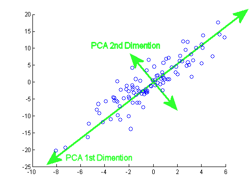
A reader might wonder, what is special about projecting bag-of-word vectors onto the top eigenvectors of covariance matrix? How does it help to extract the most informative part of original data? This is illustrated on a 2-dimensional picture below, where the blue points are 2-dimensional (for simplicity) observations.

The eigenvectors of covariance matrix have a special property that they point towards the directions of the most variance within the data. As you can see on the picture, the 1st dimension vector points towards the direction of the highest variance and the 2nd dimension vector points towards the highest variance in the subspace, orthogonal to the 1st vector. Thus, projecting onto top eigenvectors preserves maximum variance, and roughly speaking, capturing more variance means capturing more information to analyze.

Graph#1: Exponential Decay 3 Graph#2: Exponential Decay 7
Another question is how to choose the number of top eigenvectors to project on? According to my experience, a good way to choose it to plot the eigenvalues and find the point on the plot, where the eigenvalues start to decay exponentially. The eigenvalue plots for two different datasets (left and right) are illustrated on the charts above. On the left chart the point of exponential decay is 3, and on the right chart it is 7, which means that one should select 3 top eigenvalues for the left dataset and 7 for the right one. Also, you should think out of the box and see if PCA in itself is an appropriate method for your problem. With the example above, the left plot of eigenvalues shows a fast exponential decay, thus PCA is great for that problem. However, the eigenvalues on the right decay is almost linear, so PCA is not recommended.
Finally, after you have computed the low-dimensional PCA projection of your bag-of-words vectors, you can use this projection instead of original emails in classification algorithms, such as Logistic Regression or Support Vector Machine to classify the emails as spam/not spam. When projections are used instead of original emails, algorithm training will be much faster and overfitting will be reduced.
Like this article? Subscribe to our weekly newsletter to never miss out!


