An Introduction to Markov Chains Using R

Analytics has become an integral part of our daily lives. We don’t even realize how analytics is driving our decisions, our activities, our interests, our shopping behavior and more. Companies are using analytics to identify potential acquisition opportunities, their future market performances, customer behavior and many other areas. One such important use case of analytics is comparing the future performances of companies.

Let’s take a small scenario and see how analytics can help us make informed decisions based on statistically driven models. Imagine a private equity company that wants to invest in one of two chocolate brands. Before investing any money, our team at Prescriptive Analytics seeks to understand how the market share of each of the brands is going to move in the near future and in the long term. We know the current market share of each of the brands; however, we want to understand what the market share will be in subsequent months. So, how do we estimate the market share of each of the brands?

This scenario is perfect for the application of Markov Chains.

According to Paul Gagniuc’s Markov Chains: From Theory to Implementation and Experimentation,

Now, let’s break down the above statements one by one and define a Markov Chain really means. We will start with the third statement and then gradually move to the first one.

Any random process is known to have the Markov property if the probability of going to the next state depends only on the current state and not on the past states.

From the above equation, a Markov property would mean that movement from X(t) to X(t+1) will depend only on X(t), – the current state – and not on the preceding states. For example, if we were to estimate the market share of a company in the next quarter, it would depend only on the market share in the current quarter and not those of previous quarters.

The memoryless property, to put in a simpler manner, means that the Markov process doesn’t store any property or memory of its past state. From our market share example, it would mean that a Markov process doesn’t store any information on previous quarters.

If a Markov process operates within a specific set of states, it is called a Markov Chain.

A Markov Chain is defined by three properties:

1. A state space: a set of values or states in which a process could exist
2. A transition operator: defines the probability of moving from one state to another state
3. A current state probability distribution: defines the probability of being in any one of the states at the start of the process

Markov Chains in action

Now, coming back to the chocolate example we mentioned at the beginning of this article. Let’s assume the two brands of chocolate are Cadbury and Nestle.

From the Markov Chain properties:

1. The different states of the process are as follows:
   • A customer using Cadbury brand
   • A customer using Nestle products
2. Probabilities of moving from one state to another, i.e., probability of a customer changing brands is as follows:
   • Of the Cadbury customers, there is a 60% chance that the customer will stick to the Cadbury brand; while there is a 40% chance that the customer will move to Nestle.
   • Of the Nestle customers, there is a 30% chance that the customer will move to Cadbury, and a 70% chance that the customer will remain with Nestle.
3. Current state probabilities, i.e., current market share of brands are as follows:
   • Cadbury and Nestle both enjoy an equal market share of 50% each.

If we were to calculate the market share of Cadbury for the next month, it would be the sum of the following two:

• Customers currently using Cadbury and sticking with Cadbury
• Customers currently using Nestle but moving to Cadbury

Market share of Cadbury in (t+1) month =

Current Market Share of Cadbury * Probability of customers sticking with Cadbury

+

Current Market Share of Nestle * Probability of customers switching to Cadbury

Market share of Cadbury in (t+1) month = 50%*0.6 + 50%*0.3

                                                                           = 30% + 15%

                                                                           = 45%

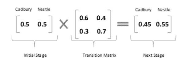
If we were to do the same using Markov Chains,

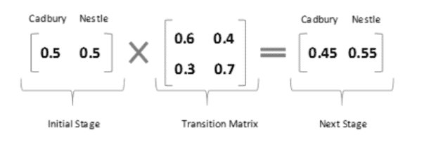
Now, calculating market share for (t+2) month =

(t+1) Market Share of Cadbury * Probability of customers sticking with Cadbury

+

(t+1) Market Share of Nestle * Probability of customers switching to Cadbury

Market share of Cadbury in (t+2) month = 45%*0.6 + 55%*0.3

                                                                           = 27% + 16.5%

                                                                           = 43.5%

If we were to do the same using Markov Chains,

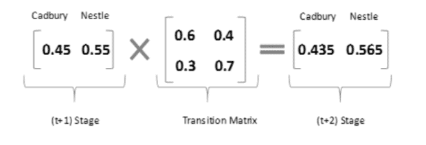
The beauty of Markov Chains is that we need not do the entire calculation for all the stages. We can directly compute market share for (t+2) stage from (t) stage.

Now, let’s take another example and try to understand the implementation using R alongside.

Let’s try to map the movement of Uber drivers in the Indian capital city of New Delhi. We can divide the city into three zones – North Delhi, South Delhi and West Delhi. The movement of drivers from one zone to another zone will depend only on their current zone. We’ve determined the following probabilities for the movement of a driver:

• Of all the drivers in North Zone, 30% will remain in North Zone, 30% will move to South zone, while the remaining 40% will go to West Zone
• In the South Zone, drivers have a 40% chance of moving to North Zone, 40% chance of staying in the South Zone;  20% drivers will move to West Zone
• Of all the drivers in West Zone, 50% and 30% will move to North Zone and South Zone, respectively; 20% will remain in West Zone

Once a driver is in a particular zone, he can either move to the next zone or stay back in the same zone. His movement will be decided only by his current state and not the sequence of past states. The state space in this example includes North Zone, South Zone and West Zone. It follows all the properties of Markov Chains because the current state has the power to predict the next stage.

Markov Chains using R

Let’s model this Markov Chain using R.

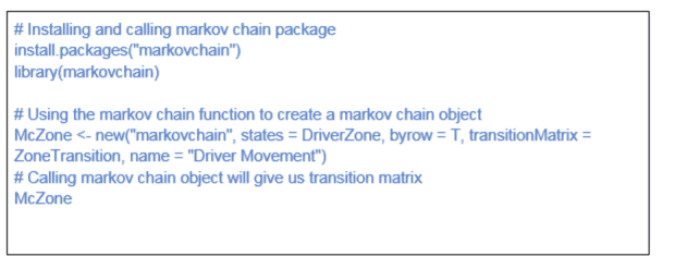
We will start by creating a transition matrix of the zone movement probabilities.

In the above code, DriverZone refers to the state space of the Markov Chain; while ZoneTransition represents the transition matrix that gives the probabilities of movement from one state to another.

There is a package in R ‘markovchain’ which can help us save time in implementing Markov Chains in R.

Now, to plot the above transition matrix we can use R package, “diagram.” The “diagram” package has a function called “plotmat” that can help us plot a state space diagram of the transition matrix in an easy-to-understand manner.

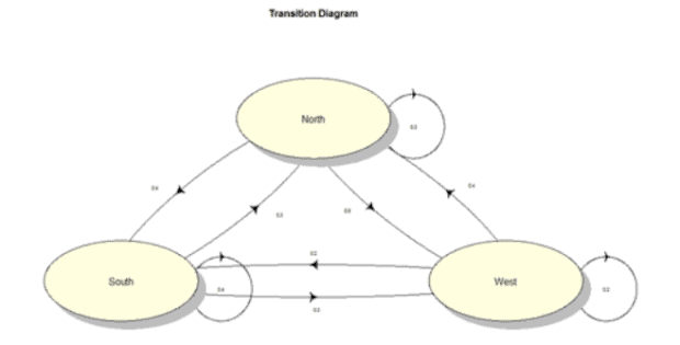
Now, the above Markov Chain can be used to answer some of the future state questions. Assuming that a driver is currently in the North Zone, what is the probability that the driver will again be in the North Zone after two trips?

A driver can reach the North Zone again in his second trip in three different ways:

1.North Zone → North Zone

Probability: P(a) = 0.3*0.3 = 0.09

2. South Zone → North Zone

P(b) = 0.4*0.3 = 0.12

3. West Zone → North Zone

P(c) = 0.5*0.4 = 0.20

Probability (North Zone in second trip) = P(a) + P(b) + P(c) = 0.09 + 0.12 + 0.20 = 0.41

Solving the same problem using Markov Chain models in R, we have:

This gives us the direct probability of a driver coming back to the North Zone after two trips.

We can similarly calculate for subsequent trips. Let’s calculate the probability of coming back to the North Zone in the third trip.

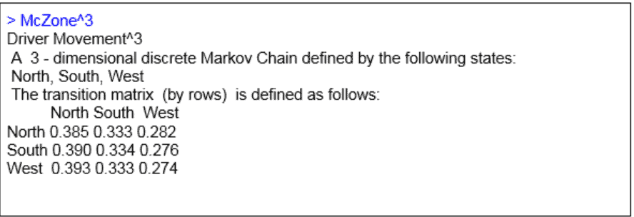
The driver has a probability of 0.385 of returning to the North Zone in the third trip.

This calculation can be done for any number of trips; however, as we try to increase n (when n is sufficiently large), the predictive power tends to go down and there comes a stage where:

P(X^(t+1)/X^(t)) = P(X^(t)/X^(t-1))

The Markov Chain reaches an equilibrium called a stationary state. In this case, the starting point becomes completely irrelevant. The stationary state can be calculated using some linear algebra methods; however, we have a direct function, ‘steadyStates’, in R, which makes our lives easier.

In the stationary state, a driver has a probability of 0.39 of ending up in the North Zone and a probability of 0.33 of reaching the South Zone.

Let’s say a driver has to complete 25 trips in a day. Will 25 trips take our Markov Chain to the stationary state?

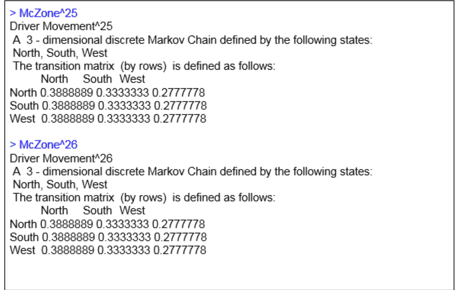
Since the probabilities in the 25th and 26th trip are coming to be equal, we can say that we have reached the stationary state.

So, if there were 50 drivers in all and each were to complete 25 trips in a day, how many of them will end up in the North Zone and South Zone?

Around 19 drivers will end up in the North Zone, 17 in the South Zone and the remaining 14 will be in the West Zone.

Markov Chains in everyday life

The above two examples are real-life applications of Markov Chains. There are plenty of other applications of Markov Chains that we use in our daily life without even realizing it. Google’s famous PageRank algorithm is one of the most famous use cases of Markov Chains. Google has indexed all websites and created a transition matrix, similar to the one we have created, but at a very large scale. Any user on the site represents one stage, and the transition matrix represents the user’s probability of moving to other sites from the current site.

Typing word prediction, information theory, queuing theory and Monte Carlo simulation are other very useful applications of Markov Chains. Markov has been used in areas of marketing, as well, with e-commerce companies are utilizing its power to define the different stages of a customer lifetime or predict customer churn probability.

It is now apparent that Markov Chains are extremely important in many areas, and it is worth becoming increasingly familiar with this type of process.

Like this article? Subscribe to our weekly newsletter to never miss out!