In a particular subset of the data science world, “similarity distance measures” has become somewhat of a buzz term. Like all buzz terms, it has invested parties- namely math & data mining practitioners- squabbling over what the precise definition should be. As a result, the term, involved concepts and their usage can go straight over the heads of beginners. So today, I write this post to give simplified and intuitive definitions of similarity measures, as well as diving into the implementation of five of the most popular of these similarity measures.
On November 25th-26th 2019, we are bringing together a global community of data-driven pioneers to talk about the latest trends in tech & data at Data Natives Conference 2019. Get your ticket now at a discounted Early Bird price!
Similarity:
Similarity is the measure of how much alike two data objects are. Similarity in a data mining context is usually described as a distance with dimensions representing features of the objects. If this distance is small, there will be high degree of similarity; if a distance is large, there will be low degree of similarity. Similarity is subjective and is highly dependent on the domain and application. For example, two fruits are similar because of color or size or taste. Care should be taken when calculating distance across dimensions/features that are unrelated. The relative values of each feature must be normalized, or one feature could end up dominating the distance calculation.Similarity is measured in the range 0 to 1 [0,1].
- Similarity = 1 if X = Y (Where X, Y are two objects)
- Similarity = 0 if X ≠ Y
Hopefully, this has given you a basic understanding of similarity. Let’s dive into implementing five popular similarity distance measures.
Euclidean distance:
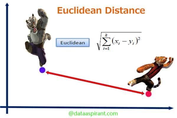
Euclidean distance is the most commonly-used of our distance measures. For this reason, Euclidean distance is often just to referred to as “distance”. When data is dense or continuous, this is the best proximity measure. The Euclidean distance between two points is the length of the path connecting them.This distance between two points is given by the Pythagorean theorem.
Euclidean distance implementation in python:
[code language="python"] #!/usr/bin/env python

from math import*

def euclidean_distance(x,y):

  return sqrt(sum(pow(a-b,2) for a, b in zip(x, y)))

print euclidean_distance([0,3,4,5],[7,6,3,-1]) [/code]
Script output:
9.74679434481
[Finished in 0.0s]
Manhattan distance:
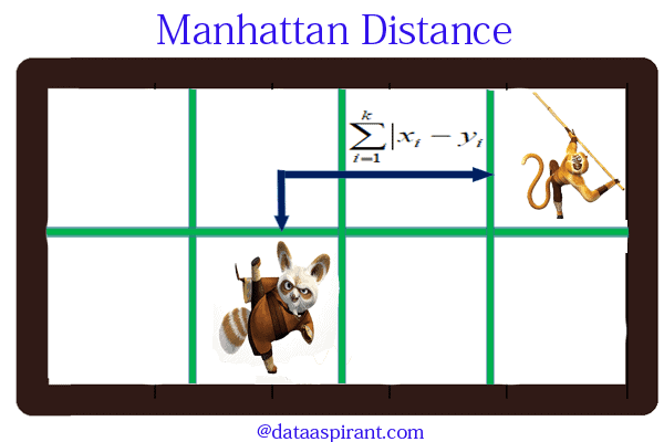
Manhattan distance is an metric in which the distance between two points is the sum of the absolute differences of their Cartesian coordinates. In simple way of saying it is the absolute sum of difference between the x-coordinates and y-coordinates. Suppose we have a Point A and a Point B: if we want to find the Manhattan distance between them, we just have to sum up the absolute x-axis and y–axis variation. We find the Manhattan distance between two points by measuring along axes at right angles.
In a plane with p1 at (x1, y1) and p2 at (x2, y2).
Manhattan distance = |x1 – x2| + |y1 – y2|
This Manhattan distance metric is also known as Manhattan length, rectilinear distance, L1 distance, L1 norm, city block distance, Minkowski’s L1 distance,taxi cab metric, or city block distance.
Manhattan distance implementation in python:
[code language="python"] #!/usr/bin/env python

from math import*

def manhattan_distance(x,y):

  return sum(abs(a-b) for a,b in zip(x,y))

print manhattan_distance([10,20,10],[10,20,20]) [/code]
Script output:
10
[Finished in 0.0s]
Minkowski distance:
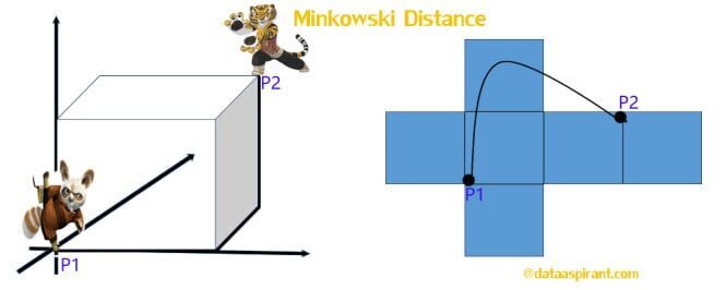
The Minkowski distance is a generalized metric form of Euclidean distance and Manhattan distance. It looks like this:
In the equation d^MKD is the Minkowski distance between the data record i and j, k the index of a variable, n the total number of variables y and λ the order of the Minkowski metric. Although it is defined for any λ > 0, it is rarely used for values other than 1, 2 and ∞.
Different names for the Minkowski difference arise from the synonyms of other measures:
- λ = 1 is the Manhattan distance. Synonyms are L1-Norm, Taxicab or City-Block distance. For two vectors of ranked ordinal variables the Manhattan distance is sometimes called Foot-ruler distance.
- λ = 2 is the Euclidean distance. Synonyms are L2-Norm or Ruler distance. For two vectors of ranked ordinal variables the Euclidean distance is sometimes called Spear-man distance.
- λ = ∞ is the Chebyshev distance. Synonym are Lmax-Norm or Chessboard distance.
Minkowski distance implementation in python:
[code language="python"] #!/usr/bin/env python

from math import*
from decimal import Decimal

def nth_root(value, n_root):

 root_value = 1/float(n_root)
 return round (Decimal(value) ** Decimal(root_value),3)

def minkowski_distance(x,y,p_value):

 return nth_root(sum(pow(abs(a-b),p_value) for a,b in zip(x, y)),p_value)

print minkowski_distance([0,3,4,5],[7,6,3,-1],3) [/code]
Script output:
8.373
[Finished in 0.0s]
Cosine similarity:
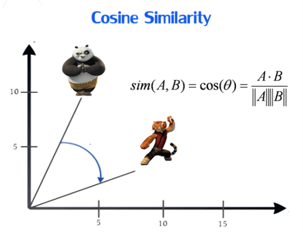
Cosine similarity metric finds the normalized dot product of the two attributes. By determining the cosine similarity, we will effectively trying to find cosine of the angle between the two objects. The cosine of 0° is 1, and it is less than 1 for any other angle. It is thus a judgement of orientation and not magnitude: two vectors with the same orientation have a cosine similarity of 1, two vectors at 90° have a similarity of 0, and two vectors diametrically opposed have a similarity of -1, independent of their magnitude. Cosine similarity is particularly used in positive space, where the outcome is neatly bounded in [0,1]. One of the reasons for the popularity of cosine similarity is that it is very efficient to evaluate, especially for sparse vectors.
Cosine similarity implementation in python:
[code language="python"] #!/usr/bin/env python

from math import*

def square_rooted(x):

   return round(sqrt(sum([a*a for a in x])),3)

def cosine_similarity(x,y):

 numerator = sum(a*b for a,b in zip(x,y))
 denominator = square_rooted(x)*square_rooted(y)
 return round(numerator/float(denominator),3)

print cosine_similarity([3, 45, 7, 2], [2, 54, 13, 15]) [/code]
Script output:
0.972
[Finished in 0.1s]
Jaccard similarity:
So far, we’ve discussed some metrics to find the similarity between objects, where the objects are points or vectors. We use Jaccard Similarity to find similarities between sets. So first, let’s learn the very basics of sets.
Sets:
A set is (unordered) collection of objects {a,b,c}. we use the notation as elements separated by commas inside curly brackets { }. They are unordered so {a,b} = {b,a}.
Cardinality:
The Cardinality of A (denoted by |A|) counts how many elements are in A.
Intersection:
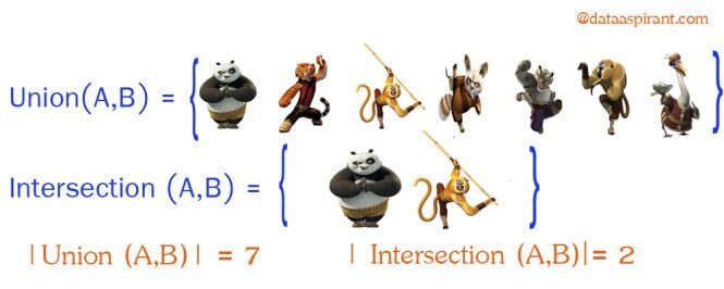
Intersection between two sets A and B is denoted A ∩ B and reveals all items which are in both sets A,B.
Union:
Union between two sets A and B is denoted A ∪ B and reveals all items which are in either set.
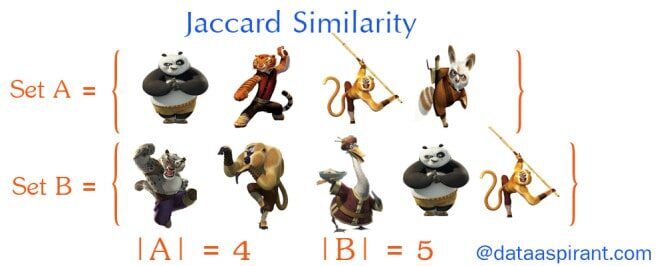
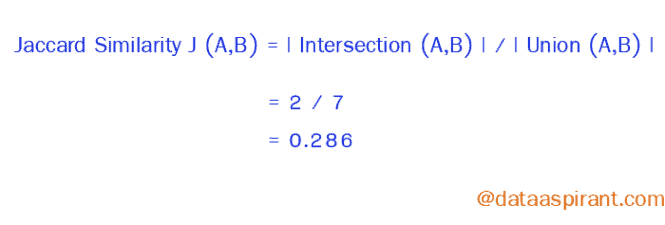
Now going back to Jaccard similarity.The Jaccard similarity measures similarity between finite sample sets, and is defined as the cardinality of the intersection of sets divided by the cardinality of the union of the sample sets. Suppose you want to find jaccard similarity between two sets A and B it is the ration of cardinality of A ∩ B and A ∪ B.
Jaccard similarity implementation:
[code language="python"]#!/usr/bin/env python

from math import*

def jaccard_similarity(x,y):

 intersection_cardinality = len(set.intersection(*[set(x), set(y)]))
 union_cardinality = len(set.union(*[set(x), set(y)]))
 return intersection_cardinality/float(union_cardinality)

print jaccard_similarity([0,1,2,5,6],[0,2,3,5,7,9]) [/code]
Script output:
0.375
[Finished in 0.0s]
Implementaion of all 5 similarity measure into one Similarity class:
file_name : similaritymeasures.py
[code language="python"]#!/usr/bin/env python

from math import*
from decimal import Decimal

class Similarity():

  """ Five similarity measures function """

  def euclidean_distance(self,x,y):

   """ return euclidean distance between two lists """

   return sqrt(sum(pow(a-b,2) for a, b in zip(x, y)))

  def manhattan_distance(self,x,y):

   """ return manhattan distance between two lists """

   return sum(abs(a-b) for a,b in zip(x,y))

  def minkowski_distance(self,x,y,p_value):

   """ return minkowski distance between two lists """

   return self.nth_root(sum(pow(abs(a-b),p_value) for a,b in zip(x, y)),p_value)

  def nth_root(self,value, n_root):

   """ returns the n_root of an value """

   root_value = 1/float(n_root)
   return round (Decimal(value) ** Decimal(root_value),3)

  def cosine_similarity(self,x,y):

   """ return cosine similarity between two lists """

   numerator = sum(a*b for a,b in zip(x,y))
   denominator = self.square_rooted(x)*self.square_rooted(y)
   return round(numerator/float(denominator),3)

  def square_rooted(self,x):

   """ return 3 rounded square rooted value """

   return round(sqrt(sum([a*a for a in x])),3)

  def jaccard_similarity(self,x,y):

   """ returns the jaccard similarity between two lists """

   intersection_cardinality = len(set.intersection(*[set(x), set(y)]))
   union_cardinality = len(set.union(*[set(x), set(y)]))
   return intersection_cardinality/float(union_cardinality) [/code]
Using similarity class:
[code language="python"] #!/usr/bin/env python

from similaritymeasures import Similarity

def main():

  """ main function to create Similarity class instance and get use of it """

  measures = Similarity()

  print measures.euclidean_distance([0,3,4,5],[7,6,3,-1])
  print measures.jaccard_similarity([0,1,2,5,6],[0,2,3,5,7,9])

if __name__ == "__main__":
  main() [/code]
The code from this post can also be found on Github, and on the Dataaspirant blog.
Photo credit: t3rmin4t0r / Foter / CC BY
